### Notebook - Demo exoSpin package

1 - Imports

The only important import you will have to do as a user is : > import exoSpin as xs (or whatever you want)

All other important packages like numpy, matplotlib are included in the exoSpin package.

# Imports
import exoSpin as xs

2 - Inputs

The main function of the exoSpin package is obliquity().

It takes as inputs path files for all parameters with a lot of data as the orbital inclination, the radius, etc.. or values as the period or the mass of the exoplanet.

For more details, go to the obliquity documentation.

# File paths & values for AB Pic b.

n = 10000 # Number of samples wanted to generate a normal distribution from only mean value and standard deviation.

exoplanet_name = 'AB Pic b'
io = 'data/io_2024.dat'
radius = 'data/rp_vrot.txt'
vsini = 'data/rp_vrot.txt'
omega = [-5,4,n]
P = 2.1
M = 10

3 - Obliquity()

The only thing you have to do is just calling the function obliquity() with all the inputs

After the calling of the function, an input user will be command: Which method of computing do you want? (easy/complex)

You just have to choose between easy or complex.

At the end you will get a nice plot of the planet’s obliquity.

x = xs.obliquity(exoplanet_name,io,radius,vsini,omega,P,M)

Initializing ExoSpin ...

-> ExoSpin Configuration

-> ExoSpin Computing

Complex method computing ...

-> ExoSpin Plot

Plot - Obliquity of AB Pic b

<Figure size 640x480 with 0 Axes>

4 - Exoplanet object

The variable x is now an Exoplanet object, so from that you can get interesting informations from it.

a) Inputs data

orbital_inclination_data = x.io
print('The data for the orbital inclination are:\n',orbital_inclination_data)

The data for the orbital inclination are:
 [ 98.10582359  98.61817799  97.9251737  ...  94.90655557  97.96513438
 103.85034903]

exoplanet_name = x.planet_name
print('The planet name is',exoplanet_name)

The planet name is AB Pic b

mass = x.mass
print('The mass of ' + exoplanet_name + ' is',mass)

The mass of AB Pic b is 10.0 jupiterMass

b) Computed data

spin_axis_data = x.ip
print('The data for the spin axis of ' + exoplanet_name + ' are: \n', spin_axis_data)

The data for the spin axis of AB Pic b are:
 [  2.37065625   2.3847321    2.48234064 ... 177.59330977 177.60180439
 177.56211114]

true_obliquity_data = x.true_obli
print('The data for the true obliquity of ' + exoplanet_name + ' are: \n',true_obliquity_data)

The data for the true obliquity of AB Pic b are:
 [100.17013052 100.9939135   99.52353419 ...  85.95676231  82.13896493
  78.58456299]

5 - Plot class

The variable x is an Exoplanet object, but it can also be mixed with a Plot class.

Indeed from Exoplanet class method like self.hist() or self.pdf(), you can compute and plot histogram or PDF (Probabilty Density Function) of exoplanet’s parameters.

After that using self.plot() will plot the computed data.

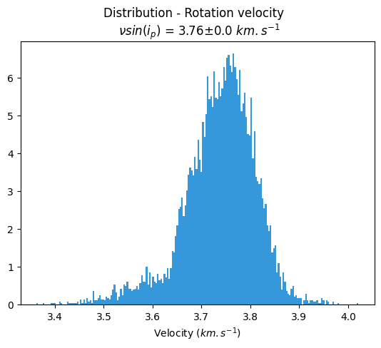
a) Histogram plot

x.hist('Rotational velocity','#3498DB').plot()

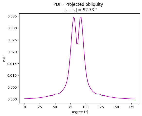
b) PDF plot

proj_pdf = x.pdf('Projected obliquity - complex','#A100A1').plot()